What a proton is depends on how you look at it, or rather on how hard you hit it. A century after Rutherford’s discovery, our picture of this ubiquitous particle is coming into focus, says Amanda Cooper-Sarkar.
Every student of physics learns that the nucleus was discovered by firing alpha particles at atoms. The results of this famous experiment by Rutherford in 1911 indicated the existence of a hard-scattering core of positive charge, and, within a few years, led to his discovery of the proton (see Rutherford, transmutation and the proton). Decades later, similar experiments with electrons revealed point-like scattering centres inside the proton itself. Today we know these to be quarks, antiquarks and gluons, but the glorious complexity of the proton is often swept under the carpet. Undergraduate physicists are more often introduced to quarks as objects with flavour quantum numbers that build up mesons and baryons in bound states of twos and threes. Indeed, in the 1960s, many people regarded quarks simply as a useful book-keeping device to classify the many new “elementary” particles that had been discovered in cosmic rays and bubble-chamber experiments. Few people were aware of the inelastic-scattering experiments at SLAC with 20 GeV electrons, which were beginning to reveal a much richer picture of the proton.
The results of these experiments in the 1960s and early 1970s were remarkable. Elastic scattering by the point-like electrons revealed the spatial distribution of the proton’s charge, and cross sections had to be modified by form-factors as a result. These varied strongly depending on how hard the proton was struck – a hardness called the scale of the process, Q2, defined by the negative squared four-momentum transfer between incoming and outgoing electrons. At high enough scales the proton broke up, a phenomenon that can be quantified by x, a kinematic variable related to the inelasticity of the interaction. Both the scale and the inelasticity could be determined from the dynamics of the outgoing electron. Physicists anticipated a complicated dependence on both variables. Studies of scattering at ever higher and lower scales continue to bear fruit to this day.
A surprise at SLAC
The big surprise from the SLAC experiments was that the cross section did not depend strongly on Q2, a phenomenon called “scaling”. The only explanation for scaling was that the electrons were scattering from point-like centres within the proton. Feynman worked out the formalism to understand this by picturing the electron as hitting a point-like “parton” inside the proton. With elegant simplicity, he deduced that the partons each carried a fraction x of the proton’s longitudinal momentum.
Gell-Mann and Zweig had proposed the existence of quarks in 1964, but at first it was by no means obvious that they were partons. The SLAC experiments established that the scattering centres had spin ½ as required by the quark model, but there were two problems. On the one hand there appeared to be not only three, but many scattering centres. On the other, Feynman’s formalism required the partons to be “free” and independent of each other, yet they could hardly be independent if they remained confined in the proton.
Painting a picture
The picture became even more interesting in the late 1970s and 1980s when scattering experiments started to use neutrinos and antineutrinos as probes. Since neutrinos and antineutrinos have a definite handedness, or helicity, such that their spin is aligned against their direction of motion for neutrinos and with it for antineutrinos, their weak interaction with quarks and antiquarks gives different angular distributions. This showed that there must be antiquarks as well as quarks within the proton. In fact, it led to a picture in which the flavour properties of the proton are governed by three valence quarks immersed in a sea of quark–antiquark pairs. But this is not all: the same experiments indicated that the total momentum carried by the valence quarks and the sea still amounts to only around half of that of the proton. This missing momentum was termed an energy crisis, and was solved by the existence of gluons with spin 1, which bind the quarks together and confine them inside the proton.
In fact, the SLAC experiments had been lucky to be making measurements in the kinematic region where scaling holds almost perfectly – where the cross section is independent of Q2. The quark–parton model had to be extended, and became the field theory of quantum chromodynamics (QCD), in which the gluons are field carriers, just like photons in quantum electrodynamics (QED). Formulated in 1973, QCD has a much richer structure than QED. There are eight kinds of gluons that are characterised in terms of a new quantum number called colour, which is carried by both quarks and the gluons themselves, in contrast to QED, where the field carrier is uncharged. The gluon can thus interact with itself as well as with quarks.
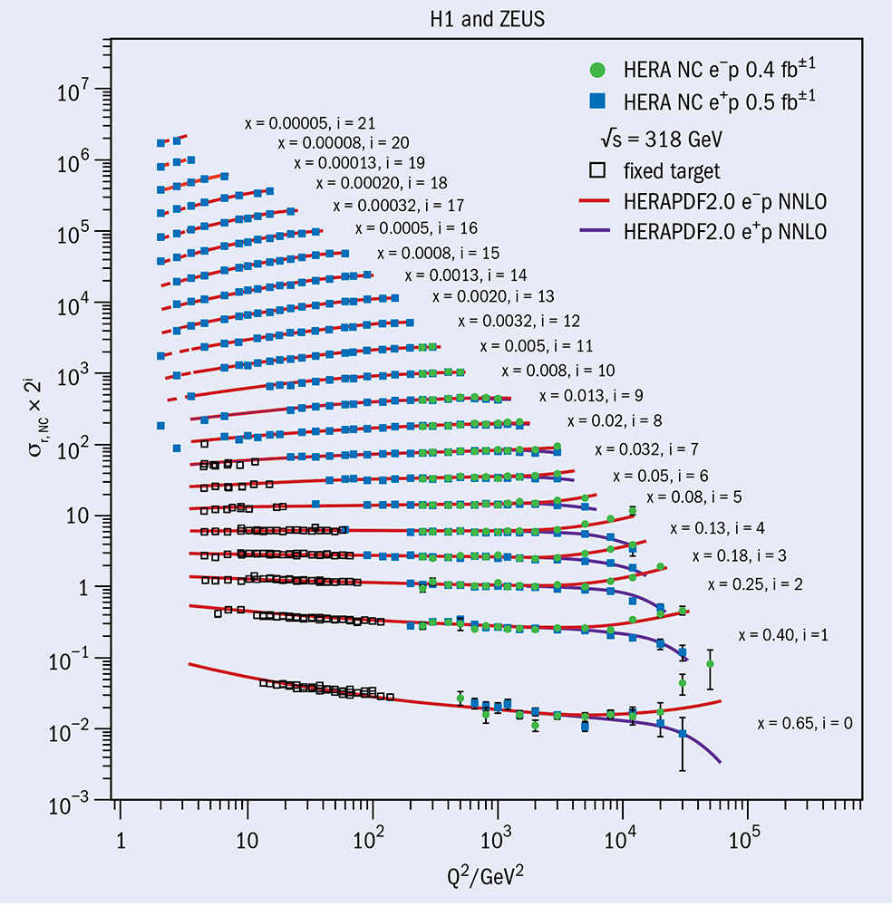
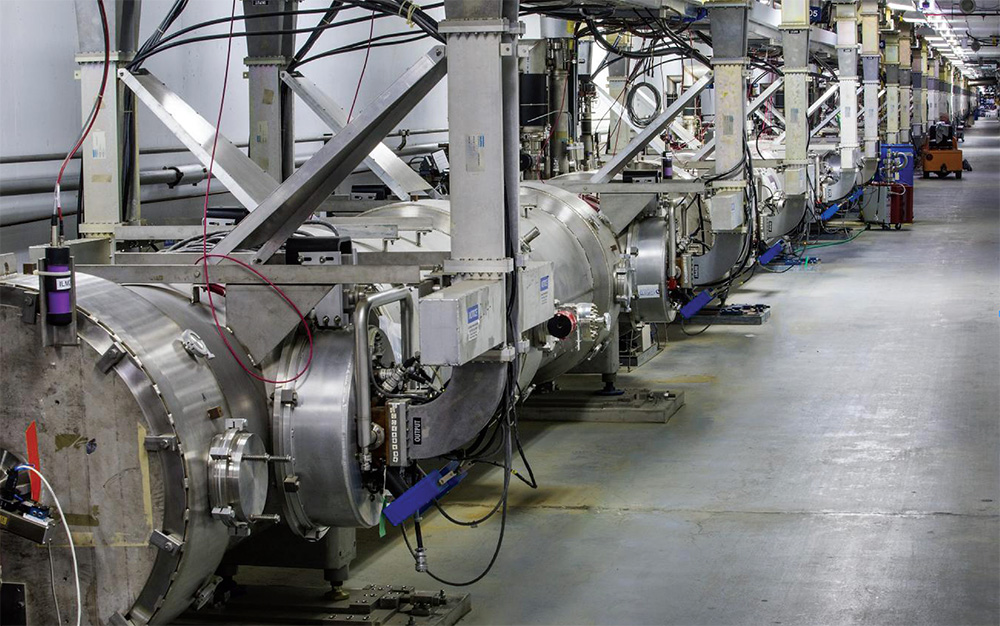
From the 1980s onwards, a series of experiments probed increasingly deeply into the proton. Deep-inelastic-scattering experiments using neutrino and muon beams were performed at CERN and Fermilab, before the HERA electron–proton collider at DESY made definitive measurements from 1992 to 2007 (figure 1). The aim was to test the predictions of QCD as much as to investigate the structure of the proton, the goal being not just to list the constituents of the proton, but also to understand the forces between them.
Meanwhile, the EMC experiment at CERN had unearthed a mystery concerning the origin of the proton’s spin (see “The proton spin crisis”), while elsewhere, entirely different experiments were placing increasingly tough limits on the proton’s lifetime (see “The pursuit of proton decay”).
The proton spin crisis
Among many misconceptions in the description of the proton presented in undergraduate physics lectures is the origin of the proton’s spin. When we tell students about the three quarks in a proton, we usually say that its spin (equal to one half) comes from the arithmetic of three spin-½ quarks that align themselves such that two point “up” and one points “down”. However, as shown in measurements of the spin taken by quarks in deep-inelastic-scattering experiments in which both the lepton beam and the proton target are polarised, this is not the case. Rather, as first revealed in results from the European Muon Collaboration in CERN’s North Area in 1987, the quarks account for less than a third of the total proton spin. This was nicknamed the proton’s “spin crisis”, and attempts to fully resolve it remain the goal of experiments today.
Physicists had to develop cleverer experiments, for example looking at semi-inclusive measurements of fast pions and kaons in the final state, and using polarised proton–proton scattering, to determine where the missing spin comes from. It is now established that about 30% of the proton spin is in the valence quarks. Intriguingly, this is made up of +65% from up-valence and –35% from down-valence quarks. The sea seems to be unpolarised, and about 20% of the proton’s spin is in gluon polarisation, though it is not possible to measure this accurately across a wide kinematic range. Nevertheless, it seems unlikely that all of the missing spin is in gluons, and the puzzle is not yet solved.
What could the origin of the remaining ~50% of the proton’s spin be? The answer may lie in the orbital angular momentum of both the quarks and the gluons, but it is difficult to measure this directly. Orbital angular momentum is certainly connected to the transverse structure of the proton. The partons’ transverse momentum must also be considered, and there is the transverse position of the partons, and the transverse, as opposed to longitudinal, spin. Multi-dimensional measurements of transverse momentum distributions and generalised parton distributions can give access to orbital angular momentum. Such measurements are underway at Jefferson Laboratory, and are also a core part of the future Electron-Ion Collider programme.
Amanda Cooper-Sarkar, University of Oxford.
Quantum considerations
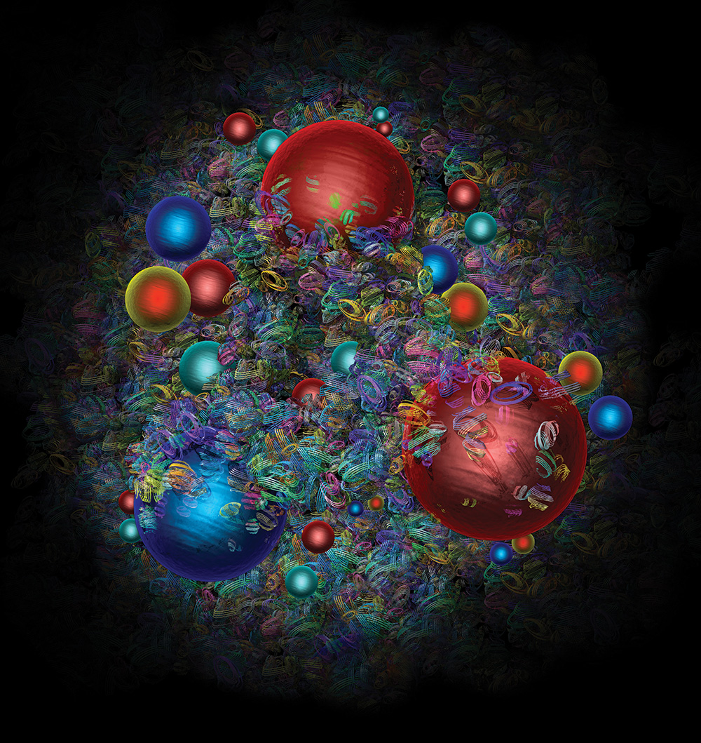
As with all quantum phenomena, what is in a proton depends on how you look at it. A more energetic probe has a smaller wavelength and therefore can reveal smaller structures, but it also injects energy into the system, and this allows the creation of new particles. The question then is whether we regard these particles as having been inside the proton in the first place. At higher scales quarks radiate gluons that then split into quark–antiquark pairs, which again radiate gluons: and the gluons themselves can also radiate gluons. The valence quarks thus lose momentum, distributing it between the sea quarks and gluons – increasingly many, with smaller and smaller amounts of momentum. A proton at rest is therefore very different to a proton, say, circulating in the Large Hadron Collider (LHC) at an energy of 7 TeV.
The deep-inelastic-scattering data from muon, neutrino and electron collisions established that QCD was the correct theory of the strong interaction. Experiments found that the structure functions which describe the scattering cross sections are not completely independent of scale, but depend on it logarithmically – in exactly the way that QCD predicts. This allowed the determination of the strong coupling “constant” αs, in analogy with the fine structure constant of QED, and it is now understood that both parameters vary with the scale of the process. In contrast with QED, the strong-coupling constant varies very quickly, from αs ~1 at low energy to ~0.1 at the energy scale of the mass of the Z boson. Thus the quarks become “asymptotically free” when examined at high energy, but are strongly confined at low energy – an insight leading to the award of the 2004 Nobel Prize in Physics to Gross, Politzer and Wilczek.
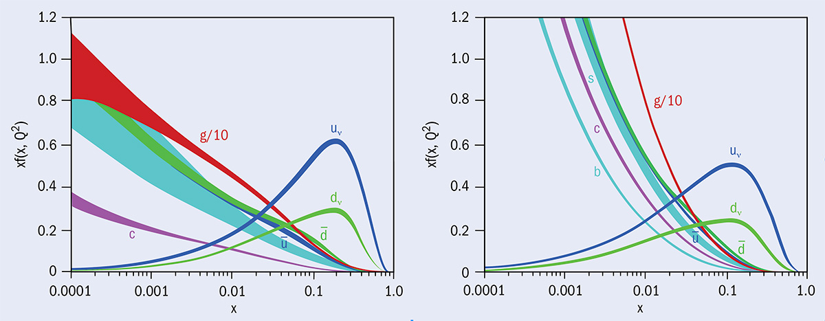
Once QCD had emerged as the definitive theory, the focus turned to measuring the momentum distributions of the partons, dubbed parton distribution functions (PDFs, figure 2). Several groups work on these determinations using both deep-inelastic-scattering data and related scattering processes, and presently there is agreement between theory and experiment within a few percent across a very wide range of x and Q2 values. However, this is not quite good enough. Today, knowledge of PDFs is increasingly vital for discovery physics at the LHC. Predictions of all cross sections measured at the LHC – whether Standard Model or beyond – need to use input PDFs. After all, when we are colliding protons it is actually the partons inside the proton that are having hard collisions and the rates of these collisions can only be predicted if we know the PDFs in the proton very accurately.
The dominant uncertainty on the direct production of particles predicted by physics beyond the Standard Model now comes from the limited precision of the PDFs of high-x gluons. Indirect searches for new physics are also affected: precision measurements of Standard Model parameters, such as the mass of the W-boson and the weak mixing angle sin2θW, are also limited by the precision of PDFs in the regions where we currently have the best precision.
The pursuit of proton decay

When Rutherford discovered the proton in 1919, the only other basic constituent of matter that was known of was the electron. There was no way that the proton could decay without violating charge conservation. Ten years later, Hermann Weyl went further, proposing the first version of what would become a law for baryon conservation. Even after the discoveries of the positron, and positive muons and pions – all lighter than the proton – there was little reason to question the proton’s stability. As Maurice Goldhaber famously pointed out, were the proton lifetime to be less than 1016 years we should feel it in our bones, because our bodies would be lethally radioactive. In 1954 he improved on this estimate. Arguing that the disappearance of a nucleon would leave a nucleus in an excited state that could lead to fission, he used the observed absence of spontaneous fission in 232Th to calculate a lifetime for bound nucleons of > 1020 years, which Georgy Flerov soon extended to > 3 × 10²³ years.
Goldhaber also teamed up with Fred Reines and Clyde Cowan to test the possibility of directly observing proton decay using a 500 l tank of liquid scintillator surrounded by 90 photomultiplier tubes (PMTs) that was designed originally to detect reactor neutrinos. They found no signal, indicating that free protons must live for > 1021 years and bound nucleons for > 1022 years. By 1974, in a cosmic-ray experiment based on 20 tonnes of liquid scintillator, Reines and other colleagues had pushed the proton lifetime to > 1030 years.
Meanwhile, in 1966, Andrei Sakharov had set out conditions that could yield the observed particle–antiparticle asymmetry of the universe. One of these was that baryon conservation is only approximate and could have been violated during the expansion phase of the early universe. The interactions that could violate baryon conservation would allow the proton to decay, but Sakharov’s suggested proton lifetime of > 1050 years provided little encouragement for experimenters. This all changed around 1974, when proposals for grand unified theories (GUTs) came along. GUTs not only unified the strong, weak and electromagnetic forces, but also closely linked quarks and leptons, allowing for non-conservation of baryon number. In particular, the minimal SU(5) theory of Howard Georgi and Sheldon Glashow led to predicted lifetimes for the decay p → e+π0 in the region of 1031±1 years – not so far beyond the observed lower limit of around 1030 years.
This provided the justification for dedicated proton-decay experiments. By 1981 seven such experiments installed deep underground were using either totally active water Cherenkov detectors or sampling calorimeters to monitor large numbers of protons. These included the Irvine–Michigan–Brookhaven (IMB) detector based on 3300 tonnes of water and 2048 5-inch PMTs and KamiokaNDE in Japan with 1000 tonnes of water and 1000 20-inch PMTs. These experiments were able to push the lower limits on the proton lifetime to > 1032 years and so discount the viability of minimal SU(5) GUTs.
However, in 1987 IMB and Kamiokande II achieved greater fame by each detecting a handful of neutrinos from the supernova SN1987a. Kamiokande II was already studying solar and atmospheric neutrinos, but it was its successor, Super-Kamiokande, that went on to make pioneering observations of atmospheric and solar neutrino oscillations. And it is Super-Kamiokande that currently has the highest lower-limit for proton decay: 1.6 × 1034 years for the decay to e+π0.
Today, the theoretical development of GUTs continues, with predictions in some models of proton lifetimes up to around 1036 years. Future large neutrino experiments – such as DUNE, Hyper-Kamiokande and JUNO – feature proton decay among their goals, with the possibility of extending the limits on the proton lifetime to 1035 years. So the study of proton stability goes on, continuing the symbiosis with neutrino research.
Chris Sutton, former CERN Courier editor.
Strange sightings at the LHC
Standard Model processes at the LHC are now able to contribute to our knowledge of the proton. As well as reducing the uncertainty on PDFs, however, the LHC data have led to a surprise: there seem to be more strange quark–antiquark pairs in the proton than we had thought (CERN Courier April 2017 p11). A recent study of the potential of the High-Luminosity LHC suggests that we can improve the present uncertainty on the gluon PDF by more than a factor of two by studying jet production, direct photon production and top quark–antiquark pair production. Measurements of the W-boson mass or the weak mixing angle will be improved by precision measurements of W and Z-boson production in previously unexplored kinematic regions, and strangeness can be further probed by measurements of these bosons in association with heavy quarks. We also look forward to possible future developments such as a Large Hadron-Electron Collider or a Future Circular Electron Hadron Collider – not least because new kinematic ranges continue to reveal more about the structure of QCD in the high-density regime.
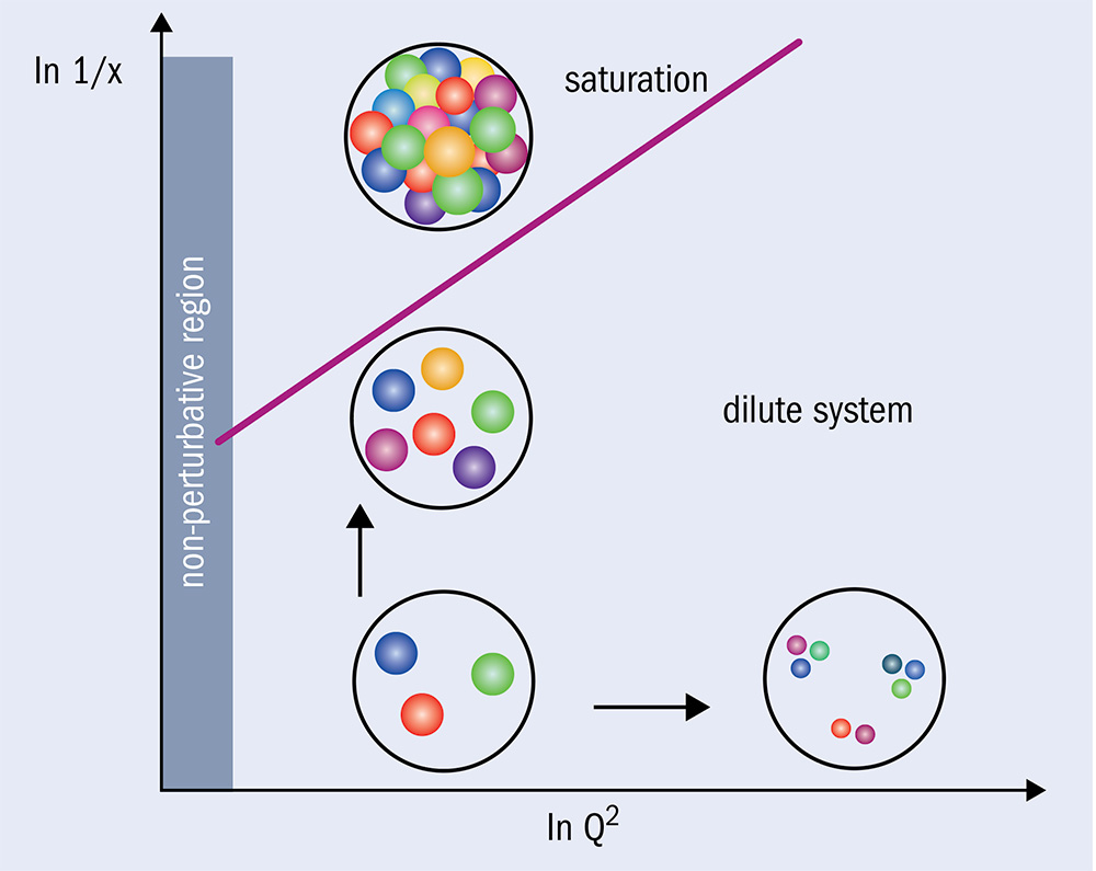
In fact the HERA data already give hints that we may be entering a new phase of QCD at very low x, where the gluon density is very large (figure 3). Such large densities could lead to nonlinear effects in which gluons recombine. When the rate of recombination equals the rate of gluon splitting we may get gluon saturation. This state of matter has been described as a colour glass condensate (CGC) and has been further probed in heavy-ion experiments at the LHC and at RHIC at Brookhaven National Laboratory. The higher gluon densities involved in experiments with heavy nuclei enhance the impact of nonlinear gluon interactions. Interpretations of the data are consistent with the CGC but not definitive. A future electron–ion collider, such as that currently proposed in the US (CERN Courier October 2018, p31), will go further, enabling complete tomographic information about the proton and allowing us to directly connect fundamental partonic behaviour to the proton’s “bulk” properties such as its mass, charge and spin. Meanwhile, table-top spectroscopy experiments are shedding new light on a seemingly mundane yet key property of the proton: its radius (see “Solving the proton-radius puzzle”).
Together with the neutron, the proton constitutes practically all of the mass of the visible matter in the universe. A hundred years on from Rutherford’s discovery, it is clear that much remains to be learnt about the structure of this complex and ubiquitous particle.
Solving the proton-radius puzzle
How big is a proton? Experiments during the past decade have called well-established measurements of the proton’s radius into question – even prompting somewhat outlandish suggestions that new physics might be at play. Soon-to-be-published results promise to settle the proton-radius puzzle once and for all.
Contrary to popular depictions, the proton does not have a hard physical boundary like a snooker ball. Its radius was traditionally deduced from its charge distribution via electron-scattering experiments. Scattering from a charge distribution is different from scattering from a point-like charge: the extended charge distribution modifies the differential cross section by a form factor (the Fourier transform of the charge distribution). For a proton this takes the form of a dipole with respect to the scale of the interaction, and an exponentially decaying charge distribution as a function of the distance from the centre of the proton. Scattering experiments found the root mean square (RMS) radius to be about 0.88 fm.
Since the turn of the millennium, a modest increase in precision on the proton radius was made possible by comparing measurements of transitions in hydrogen with quantum electrodynamics (QED) calculations. Since atomic energy levels need to be corrected due to overlapping electron clouds in the extended charge distribution of the proton, precise measurements of the transition frequencies provide a handle on the proton’s radius. A combination of these measurements yielded the most recent CODATA value of 0.8751(61) fm.
The surprise came in 2010, when the CREMA collaboration at the Paul Scherrer Institute (PSI) in Switzerland achieved a 10-fold improvement in precision via the Lamb shift (the 2S–2P transition) in muonic hydrogen, the bound state of a muon orbiting a proton. As the muon is 200 times heavier than the electron, its Bohr radius is 200 times smaller, and the QED correction due to overlapping electron clouds is more substantial. CREMA observed an RMS proton radius of 0.8418(7) fm, which was five sigma below the world average, giving rise to the so-called “proton radius puzzle”. The team confirmed the measurement in 2013, reporting a radius of 0.8409(4) fm. These observations appeared to call into question the cherished principle of lepton universality.
More recent measurements have reinforced the proton’s slimmed-down nature. In 2016 CREMA reported a radius of 0.8356(20) fm by measuring the Lamb shift in muonic deuterium (the bound state of a muon orbiting a proton and a neutron). Most interestingly, in 2017 Axel Beyer of the Max Planck Institute of Quantum Optics in Garching and collaborators reported a similarly lithe radius of 0.8335(95) fm from observations of the 2S–4P transition in ordinary hydrogen. This low value is confirmed by soon-to-be-published measurements of the 1S–3S transition by the same group, and of the 2S–2P transition by Eric Hessels of York University, Canada, and colleagues. “We can no longer speak about a discrepancy between measurements of the proton radius in muonic and electronic spectroscopy,” says Krzysztof Pachucki of CODATA TGFC and the University of Warsaw.
But what of the discrepancy between spectroscopic and scattering experiments? The calculation of the RMS proton radius using scattering data is tricky due to the proton’s recoil, and analyses must extrapolate the form factor to a scale of Q2 = 0. Model uncertainties can therefore be reduced by performing scattering experiments at increasingly low scales. Measurements may now be aligning with a lower value consistent with the latest results in electronic and muonic spectroscopy. In 2017 Miha Mihovilovic of the University of Mainz and colleagues reported an interestingly low value of 0.810(82) fm using the Mainz Microtron, and results due from the Proton Radius Experiment (pRad) at Jefferson Lab will access a similarly low scale with even smaller uncertainties. Preliminary pRad results presented in October 2018 at the 5th Joint Meeting of the APS Division of Nuclear Physics and the Physical Society of Japan in Hawaii indicate a proton radius of 0.830(20) fm. These electron-scattering results will be complemented by muon-scattering results from the COMPASS experiment at CERN, and the MUSE experiment at PSI.
For now, says Pachucki, the latest CODATA recommendations published in 2016 list the higher value obtained from electron scattering and pre-2015 hydrogen-spectroscopy experiments. If the latest experiments continue to line up with the slimmed-down radius of CREMA’s 2010 result, however, the proton radius puzzle may soon be solved, and the world average revised downwards.
Mark Rayner, CERN.
Further reading
R Devenish and A Cooper-Sarkar 2004 Deep Inelastic Scattering (Oxford University Press).
J Campbell et al. 2018 The Black Book of Quantum Chromodynamics (Oxford University Press).