Physics Archives – Page 130 of 142

Second postcard from the island of stability

cernsuper1-10-01 — Fig.1a: Prominent decay chains observed in the reactions calcium-48 and plutonium-244.

Half a century ago, Edwin McMillan and Glenn Seaborg of Berkeley were awarded the 1951 Nobel Prize for Chemistry for their elucidation in the early 1940s of the first ‘transuranic’ nuclei – synthetic radioactive nuclei heavier than uranium, which conventionally marks the end of the Periodic Table of nuclei. Since then, patient work has discovered a series of highly unstable superheavy nuclei, but a fundamental nuclear prediction said that an “island of stability” would eventually be reached.

The article “First postcard from the island of nuclear stability” reported the first results obtained at the Joint Institute for Nuclear Research (JINR), Dubna, on the synthesis of superheavy nuclei in fusion reaction induced by a calcium-48 beam. Targets of plutonium isotopes with mass numbers 242 and 244 furnished new nuclides, notably with 114 protons, and their subsequent alpha decays, terminated by spontaneous fission.

cernsuper1A-10-01 — Fig.1b: Prominent decay chains observed in the reactions calcium-48 and curium-248.

The conclusion was that in these reactions the even-odd isotopes of element 114 had been produced following the emission from an intermediate compound nucleus of three neutrons, together with gamma rays. The formation cross-sections were very small (~1 pb). The radioactive properties of these nuclides (energies and half-lives) demonstrated the existence of a new region of nuclear stability, which had been predicted earlier as due to nuclear shell effects.

The experiments were performed in the Flerov Laboratory of Nuclear Reactions (JINR) in collaboration with the Lawrence Livermore National Laboratory (LLNL), GSI (Darmstadt), RIKEN (Saitama), the Comenius University (Bratislava) and the University of Messina (Italy) (Oganessian et al. 1999a and 1999b).

During work carried out in June to November 1999, a plutonium-244 target was bombarded by a calcium-48 beam (total beam dose about 10¹⁹ ions). Two more identical decay chains were observed (Oganessian et al. 2000a and 2000b). Each consisted of two sequential alpha decays that were terminated by spontaneous fission characterized by a large energy release in the detectors (figure 1a).

Following the trail

The new alpha-decay energies are slightly higher than in the previous case and the total decay time is shorter (about 0.5 min). The probability that the observed decays are due to random coincidences is less than 5 x 10^-13.

Both events were observed at a beam energy that corresponded to a compound-nucleus excitation energy of 36-37 MeV. Here, the most probable de-excitation channel of the hot nucleus 292/114 corresponds to the emission of four neutrons together with gamma rays. Taking this into account, the new decay chains had to be attributed to the decay of the neighbouring even-even isotope of element 114 with mass 288.

To check this conclusion, further experiments continued with a curium-248 target (Oganessian et al. 2001). In Dimitrovgrad, Russia, 10 mg of the highly enriched isotope was produced. More such target material was provided by LLNL.

Changing the target from plutonium-244 to curium-248, while maintaining all other experimental conditions, makes the fusion reaction lead to the formation in the four-neutron evaporation channel of a new heavier nucleus, this time with 116 protons and mass 292. Its probable alpha decay leads to a daughter nucleus, the isotope 288/114 previously synthesized in the calcium-48/plutonium-244 reaction via the four-neutron evaporation channel. Thus, after the decay of the 292/116 nucleus, the whole decay chain of the daughter 288/114 nucleus should be observed (figure 1a).

The experimental conditions

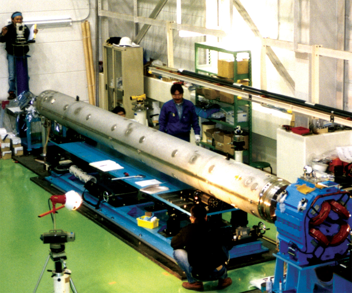
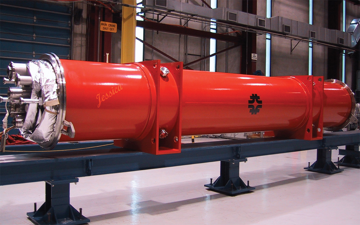
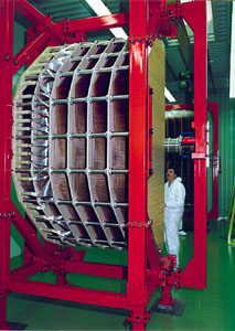
In the original experiment, the recoil atoms were separated in flight from the beam particles and the products of incomplete fusion reactions analysed by the Dubna gas-filled recoil separator (DGFRS).

cernsuper2-10-01 — Fig. 2: Energy spectra of alpha particles and spontaneous fission fragments, obtained in reactions of calcium-48 with plutonium-244 and curium-248 targets. The half-lives of the nuclei obtained from the time distributions of the observed events are also shown.

Separated heavy atoms were implanted into a 4 x 12 cm² detector located in the focal plane 4 m from the target. The front detector was surrounded by side detectors in such a way that the entire array resembled a “box” with an open front. This increased the detection efficiency of alpha particles from the decay of an implanted nucleus to 87% of the total solid angle.

For each atom implanted in the sensitive layer of the detector, the velocity and energy of the recoil were measured, as well as the location on the detector area. If the nucleus of the implanted atom emitted an alpha particle or fission fragments, the latter were detected in a strict correlation with the implant on the position sensitive surface of the detector.

Usually the experiments are performed using a continuous beam. However, for the synthesis of element 116, these conditions were changed. After implantation in the front detector of a heavy nucleus with the expected parameters and the subsequent emission of an alpha particle with energy above 10 MeV (the two signals are strictly correlated in position), the accelerator was switched off and the subsequent decays took place without the beam.

The measurements performed immediately after turning off the accelerator beam showed that the counting rate of alpha particles (energy above 9.0 MeV) and fission fragments from spontaneous fission in a 0.8 mm position window, defined by the position resolution of the detector, amounts to 0.45 per year and 0.2 per year respectively. Random coincidences imitating a three-step 1-3 min decay chain of the nucleus 288/114 are practically impossible, even for a single event.

Decay chains

In such conditions at a beam dose of 2.3 x 10¹⁹ ions, three decay chains of element 116 were registered (figure 1b). After the emission of the first alpha particle (energy 10.53 ± 0.06 MeV), the sequential decay was recorded with the beam turned off.

As can be seen from figure 1b, all decays are strictly correlated; the five signals in the front detectors – the recoil nucleus, three alpha particles and fission fragments – deviate by no more than 0.6 mm.

The alpha-particle energies and the half-lives of the nuclei in the three decay chains, the first alpha decays and those detected after the accelerator was switched off are all consistent between each other within the limits of the detector energy resolution (60 keV) and the statistical fluctuations in the decay time of the events.

All of the detected decays following the first 10.53 MeV alpha particle agree well with the decay chains of 288/114 observed in the earlier reaction (see figure 1a). Thus it is reasonable to assign the observed decay to the nuclide 292/116, produced via the evaporation of four neutrons in the complete fusion reaction using curium-248.

The energy spectrum of the three events corresponding to the nucleus 292/116, and the five events corresponding to the alpha decay of the daughter nuclei 288/114 and 284/112, as well as the summed energy of the fragments from five events of spontaneous fission of the nucleus 280/110, obtained in the experiments with the plutonium and curium targets, are shown in figure 2.

Well defined decay energy

As expected for even-even nuclei, the experimentally observed alpha decay is characterized by a well defined decay energy, corresponding to the mass difference between the mother and daughter nuclei. The time distribution of the signals in the decay chains follows an exponential decay law. The half-lives for each nucleus are also shown in figure 2.

cernsuper3-10-01 — Fig. 3: Calculated and experimental alpha-decay energy and half-life relationships for even-even isotopes with more than 100 protons. The data, obtained in the reactions of calcium-48 with plutonium-244 and curium-248 targets, are shown as black squares.

For allowed alpha transitions (even-even nuclei) the decay energy and probability (half-life) are connected by the well known Geiger-Nuttall relation. This is strictly fulfilled for all currently known 60 nuclei heavier than lead 208 for which data are available. Figure 3 shows the calculated and experimental data for nuclei with more than 100 protons and the data from the present experiment on the synthesis of nuclei with 112, 114 and 116 protons.

Owing to the high precision of the alpha-particle energy measurements (resolution 0.5%), any other interpretation of the atomic numbers of the observed decays would have been in strong contradiction with the general characteristics of alpha decay.

Finally, in the spontaneous fission of 280/110, the fission fragment energy measured in the detectors amounted to 206 MeV. This corresponds to a mean fission fragment kinetic energy of 230 MeV (taking into account the energy loss in the dead layer of the detector), which is characteristic of the fission of a rather heavy nucleus. In the thermal-neutron fission of uranium, the corresponding energy is 168 MeV.

Increased stability

Comparing spontaneous fission and alpha-decay half-lives for nuclei with 110 and 112 protons with earlier data for the lighter isotopes of these elements shows a significant increase in the stability of heavy nuclei with increasing neutron number. The addition of 10 neutrons to the 270/110 nucleus makes the half-life a hundred thousand times as long. The isotopes of element 112 with masses 277 and 284 exhibit a comparable effect.

Comparing the experimental alpha-decay energy values with those calculated in different models shows that the difference between experiment and theory is in the range ±0.5 MeV. Without going into any detailed analysis, the conclusion can be drawn that theoretical models developed during the last 35 years and predicting the decisive influence of nuclear structure on the stability of superheavy elements are well founded, not only qualitatively but also, to a certain extent, quantitatively.

This increased stability significantly extends research in the region of superheavy elements, opening up the study of such areas as their chemical properties and the measurement of their atomic masses. The development of the experimental techniques will make it possible to advance into the region of even heavier nuclei – expect more postcards in the years to come!

The experiments were carried out in collaboration with the Analytical and Nuclear Chemistry Division of the Lawrence Livermore National Laboratory.

*Evidence for the superheavy nucleus 118, reported by Berkeley scientists in 1999 has been retracted.

Weighing the antiproton

cernanti1-10-01 — Members of the ASACUSA antiproton experiment at CERN. ASACUSA involves physicists from Bulgaria, CERN, Denmark, France, Germany, Hungary, Japan, the Netherlands, Russia and the UK.

Knowing the exact charges and masses of the protons, electrons and neutrons that constitute matter is evidently of fundamental importance for the entire edifice of particle physics. Furthermore, once we know these, we know, according to CPT-symmetry, the values for the corresponding components of the antiworld. Given the fact that we already know the particle values very precisely, should we even bother making the measurements for antiparticles?

Such an omission could hardly be more risky. The CPT theorem – which says that all observed phenomena will remain unchanged if we replace particles by antiparticles, invert their motions, and reflect everything in a mirror – is based on falsifiable assumptions. In a universe as old and as big as the one we see, there is time and space enough for even minute deviations from perfect CPT symmetry to become observable, perhaps even to predominate.

Warning messages

Nature even seems to be sending us warning messages in this respect: having provided a full kit of parts for making a large scale universe that is matter-antimatter symmetric, the one that it in fact assembles from these parts is completely asymmetric. Of course we have explanations for this imbalance, but they are not beyond question. Even worse, the CPT theorem itself rests, as T D Lee notes, “on a foundation which has to be unsound, at least at the Planck length (10^-33 cm – the measurement precision when quantum fluctuations begin to have gravitational implications), and maybe at a much larger distance” (T D Lee 1995 The Discovery of Nuclear Antimatter Italian Physical Society Conf. Proceedings vol. 53 eds L Maiani and R A Ricci). The symmetry between matter and antimatter, he concludes, “must rest on experimental evidence”.

How then can we measure the antiproton charge, Q, and mass, M, with very high precision? For the proton, as few particle physicists realize, the charge is measured by taking an acoustic cavity containing sulphur hexafluoride and trying to make it “sing” in tune with an oscillating electric field. The extent to which it does not can then be interpreted as a limit on the net charge of bulk matter: if the proton’s and the electron’s charges were not very close, sulphur hexafluoride would sing louder than it does.

In the case of electrons the charge, e, is no longer obtained, as one might think, from a Millikan-type oil drop experiment, but by combining measurements of the Josephson constant, e/h, and the fine structure constant, a, which appears as a scale factor for all energy levels in the hydrogen atom and is proportional to e²/h. That way, not only e but also h, the Planck constant, can be determined.

As antisulphur hexafluoride is not exactly common on Earth (and also for want of a suitable container for it), we must look elsewhere for a value of the antiproton’s charge. The electron e/h and e²//h experiments give us a clue as to how this can be done.

Some years ago the antiproton’s Q/M value was measured relative to that of the proton’s by the Harvard group at CERN’s LEAR low-energy antiproton ring (R A Ricci 1999 Phys. Rev. Lett. 82 3198) to the staggering precision of 9 parts in 10¹¹. This value was not deduced from measurements of the curvature of its trajectory in a magnetic field (such a measurement could never be made with a better error margin than a few parts per thousand) but by tickling it with microwaves to determine its cyclotron frequency, Q/M ¥ B, in the field B.

In physics we build on what we know, not on what we don’t know, so we are not allowed to assume that unknown CPT violations do not scale Q and M proportionately, leaving Q/M unchanged. The question of values for the charge and mass individually was therefore still open. An independent measure of some other combination of Q and M was needed, just as the fine structure constant gives a different combination of e and h above to the one given by the Josephson constant. What better than the Rydberg constant of the antiproton, which is proportional to Q²M?

For this we need an atom in which the antiproton orbits a nucleus, as the electron does in hydrogen. A good candidate (indeed the only one available at present) is the antiprotonic helium atom (an antiproton and an electron orbiting an alpha particle nucleus), easily created by stopping antiprotons from CERN’s antiproton decelerator in helium gas.

By probing this atom with laser beams, ASACUSA can measure a number of optical transition frequencies between pairs of antiproton orbital states with principal and angular momentum quantum numbers (n, L) differing by one (see “Thinking about antiprotonic helium” below). In sharp contrast with the case of electrons in ordinary helium and of hydrogen, these take values around 35-40 when the almost stationary antiproton is captured into an atomic orbit by a helium nucleus (see “Thinking about antiprotonic helium” below). Every such transition of the antiproton in this atom has the antiproton Rydberg constant as a common scale factor.

Now, of course, much of the art of high-precision experimentation lies in accounting for small systematic errors. Stopping the antiprotons in very cold (6 K) helium reduced those due to the Doppler effect severely. The major remaining systematic effect was the so-called density shift arising from the buffeting that the antiprotonic atom suffers from neighbouring ordinary helium atoms. On the theoretical side, the difficulty is that antiprotonic helium is a three-body system, not a two-body system like hydrogen, requiring sophisticated computer calculations.

Among the many transition frequencies measured, the experimenters therefore selected those with the most favourable experimental and theoretical conditions. Instead of trying to work out a value for the Rydberg constant, and combining it with the Q/M value, the equivalent procedure was adopted, asking the theorists to estimate how much the proton values for Q and M used in their calculations had to be changed to give the experimental frequencies, under the 9 parts in 10¹¹constraint given by the Harvard Q/M ratio. This could be interpreted as a confidence limit on the charge and mass relative to those of the proton.

The result was that if there is any difference between the antiproton Q or M and the proton’s value, it is, with a 90% confidence level, less than 6 parts in 10⁸. This constraint is about 10 times as tight as that obtained by the same procedure at LEAR and a thousand times as tight as that obtained without using antiprotonic helium.

Can we stop here? No. As has been often pointed out, in science we can never verify concepts (like CPT symmetry) with absolute finality – there is always the possibility that still more precise measurements, or measurements of new quantities, will falsify them. This is why the ASACUSA group is now planning further improvements to its laser system that will push the limit to a few parts in one billion, and why it is now also measuring the magnetism of the antiproton to a few parts in 10⁵ or better by flipping the electron’s spin in its orbital magnetic field. The first results are being displayed prominently in the photograph by Hiroyuke Torii of Tokyo.

Thinking about antiprotonic helium

cernanti2-10-01 — The energy levels of the antiprotonic helium atom.

A useful starting point for thinking about antiprotonic helium is the semiclassical picture of the Bohr hydrogen atom usually presented in undergraduate textbooks. It has now been established that if the antiproton approaches an ordinary helium atom slowly enough, it readily replaces one of its electrons, entering an orbit with the same semiclassical radius (some 10⁵nuclear radii – well beyond the range of annihilation – producing strong interactions) and therefore the same binding energy of about 39.5 eV.

As a first approximation we assume (as is also done in textbooks for ordinary helium) that it does not interact with the remaining electron, but that this nevertheless partially screens the nuclear charge to the value 1.7e instead of 2e. This approximation is adequate to reveal the general properties of the spectrum.

The total (kinetic plus potential) energy in such hydrogen-like atoms is quantized with energy levels E_n = -E_R/n², where E_R is the energy equivalent of the antiproton_helium Rydberg constant. Doing the calculations we then easily find that n is about 38 for E_n = 39.5 eV, and that the de Broglie wavelength of the antiproton is n times smaller than that of the electron (0.05 nm), justifying our semiclassical assumption. The electron itself is fully quantum mechanical as it was before the antiproton approached.

The figure “Energy levels” shows a schematic energy level diagram for the atom. Evidently the antiproton is in a very highly excited state. Hold the figure vertically in front of you and the n = 1, L = 0 ground state energy of about -60 keV will be found way off the page to the left and a few hundred metres underground!

Now one might have thought that if, during its nanosecond-long approach to the atom, the antiproton had been able to displace the first electron so easily, it would within a few more nanoseconds just as easily have ejected the second one and that the atom (right thumbnail sketch) would quickly become a positive ion (left thumbnail sketch).

The most important characteristic of this atom is that energy and angular momentum conservation prevents this from happening, at least immediately. Instead, the antiproton de-excites spontaneously (black arrows) through a chain of metastable states, emitting optical-frequency (2 eV or 600 nm) photons as it goes with microsecond-scale lifetimes.

Only when it arrives at one of the red states do the energy and angular momentum transfers become favourable for removing the second electron and so for changing the neutral atom into a positive ion. Once this happens the antiproton’s fate is sealed – such ions are very unstable in collisions with ordinary helium atoms, and these soon send the antiproton into the nucleus, where it annihilates.

ASACUSA’s trick is to stimulate transitions to green states with a tunable laser beam, and to detect the resonance condition between the laser beam and the atom by the ensuing annihilation.

LHC insertions: the key to CERN’s new accelerator

US contribution to the LHC – superconducting separator dipole made by the US Brookhaven Laboratory. Credit: CERN

When the machine runs in collider mode, one should forget the lattice,” said Norbert Siegel. “Where it all happens is at the interaction points.” Siegel is leader of the CERN group responsible for Large Hadron Collider LHC superconducting magnets other than those of the machine’s main lattice. Like other accelerators and colliders, the LHC’s magnets can be divided into two categories. Lattice magnets keep protons on course and are responsible for maintaining stable circulating beams. The rest go by the name of insertion magnets, performing specific tasks such as final focus before collision, beam cleaning, injection and extraction.

Inner triplets

For the LHC, the most complex insertion magnets are the eight so-called inner triplets that will squeeze the proton beams and bring them into collision in the centre of the four LHC experiments. The inner triplets are placed symmetrically at a distance of 23 m on either side of the interaction points, and each forms a cryogenic unit about 30 m long. They consist of four low-beta quadrupole magnets, so-named because their job is to minimize the beta-function, which is proportional to beam size, at the interaction point. Because of the special job they have to do and their proximity to the interaction points, the inner triplet magnets will be subject to unusually high heat loads. This means that a superfluid helium heat exchanger of unprecedented scale is required to keep them at their 1.9 K operating temperature.

Quadrupole on the test bench — Japan: the first KEK-built, full-length prototype low-beta quadrupole on the test bench. Credit: CERN

The inner triplets are being provided as part of the US and Japanese contributions to the LHC project. They will use two types of quadrupole, along with various corrector magnets that are being supplied by CERN. One type of quadrupole is being developed at Japan’s KEK laboratory, the other at the US Fermilab, which also has the task of integrating all of the components into their cryostats. After a successful development programme using short model magnets, full- size low-beta quadrupoles have been made and were tested in May.

The first piece of hardware built by the US–LHC project, which coordinates the US contribution to the accelerator, arrived at CERN from Fermilab last year (CERN Courier November 2000 p40). A heat exchanger test unit, it had the job of verifying the design of the inner triplet cooling system. Existing data on heat exchangers of this scale being scarce, the final inner triplet design had to wait until the test unit was put through its paces at CERN, one of the few places in the world with the capacity to provide superfluid helium at the necessary flow rate. With the tests reaching a successful conclusion, the design has now been frozen and inner triplet production started at Fermilab in July. The first inner triplet is scheduled to arrive at CERN by the end of 2002.

Dedicated separators

As well as bringing the accelerator’s counter-rotating beams together, LHC insertion magnets also have to separate them after collision. This is the job of dedicated separators, and the US Brookhaven Laboratory is developing superconducting magnets for this purpose. Brookhaven is drawing on its experience of building the Relativistic Heavy Ion Collider (RHIC), which like the LHC is a superconducting machine. Consequently, these magnets will bear a close resemblance to RHIC’s main dipoles. Following a prototyping phase, full-scale manufacture has started at Brookhaven and delivery of the first superconducting separator magnets to CERN is fore seen before the end of the year.

Twin-aperture quadrupole — Canada: the first series production twin-aperture quadrupole produced by the TRIUMF laboratory, Vancouver, with ALSTOM Canada. Credit: CERN

All LHC insertions include dispersion suppressors and matching sections. The dispersion suppressors will limit the variation of beam position at the collision points caused by a spread in particle momenta, while the matching sections tailor the beam size in the insertions to the acceptance of the machine’s lattice. Dedicated insertion quadrupoles of various designs have been developed and optimized by CERN to fulfil the aperture, space and magnetic strength requirements for these tasks. All are now at the production stage in European industry, with the first due for delivery at the beginning of 2002.

Other magnets

All of the magnets discussed above are superconducting. The LHC will, however, make use of room-temperature magnets in several of its insertions. These are being provided as part of the Russian and Canadian contributions to the LHC, and they include special quadrupoles and dipoles for the beam-cleaning insertions, and beam injection and ejection magnet systems that include fast kicker magnets and steel septum magnets. The septa are all being provided by the Russian IHEP laboratory in Protvino near Moscow, where production is well under way. In the cleaning insertions, which remove beam halo particles from the circulating beams, magnets must operate at room temperature due to the harsh radiation environment. Separation dipoles for these insertions are being made by the Russian Budker Institute of Nuclear Physics in Novosibirsk, while double-aperture quadrupoles are being provided by Canada’s TRIUMF laboratory.

Quadrupole ready for measurements — US: a cryostated full-length low-beta quadrupole ready for measurements at Fermilab. Credit: CERN

Finally, there is one kind of insertion magnet that plays no role in the effective working of the LHC as a collider – the huge magnet systems of the four experiments. Their magnetic fields have an influence on the beams’ trajectories and have to be compensated for by orbit compensation magnets.

Production of all of the LHC insertion magnets is now well under way. Their preparation and installation in the tunnel, along with integration with other LHC systems, such as cryogenics, vacuum and power, provide challenging work for the years ahead. When that is over and the LHC is complete, it will be a phenomenally complex machine. However, as Norbert Siegel points out, once the LHC is running, attention will be diverted from the machine, as all eyes turn to the four main experimental insertions – the key to a better under standing of our universe.

Fifty years of the renormalization group

Quantum field theory is the calculus of the microworld. It consists principally of a combination of quantum mechanics and special relativity, and its main physical ingredient – the quantum field – brings together two fundamental notions of classical (and non-relativistic quantum) physics – particles and fields.

For instance, the quantum electromagnetic field, within appropriate limits, can be reduced to particle-like photons (quanta of light), or to a wave process described by a classical Lorentz field. The same is true for the quantum Dirac field.

Quantum field theory (QFT) , as the theory of interacting quantum fields, includes the remarkable phenomenon of virtual particles, which are related to virtual transitions in quantum mechanics. For example, a photon propagating through empty space (the classical vacuum) undergoes a virtual transition into an electron-positron pair. Usually, this pair undergoes the reverse transformation: annihilation back into a photon. This sequence of two transitions is known as the process of vacuum polarization (figure 1(a)). Hence the vacuum in QFT is not an empty space; it is filled by virtual particle-antiparticle pairs.

cernquan1_9-01 — Fig 1. (a) A photon propagating through empty space (the classical vacuum) undergoes a virtual transition into an electron-positron pair. Feynman diagrams are the classical method for displaying such processes. (b) and (c) show such diagrams for the scattering of an electron and a proton.

Another example of vacuum polarization is the electromagnetic interaction between two electric charges (e.g. between two electrons, or between a proton and an electron). In QFT, rather than a Coulomb force described by a potential, the interaction corresponds to an exchange of virtual photons, which, in turn, propagate in space-time accompanied by virtual electron-positron pairs (figure 1(c)). The theory of the interaction of quantum fields of radiation (photons) and of quantum Dirac fields (electrons and positrons) formulated in the early 1930s is known as quantum electrodynamics.

QFT calculation usually results in a series of terms, each of which represents the contribution of different vacuum-polarization mechanisms (illustrated by Feynman diagrams). Unfortunately, most of these terms turn out to be infinite. For example, electron-proton scattering, as well as Feynman diagram 1(b) (Møller scattering), also includes radiative corrections (figure 1(c)). This last contribution is infinite, owing to a divergence of the integral in the low wavelength/high-energy region of possible momentum values of the virtual electron-positron pair. One such infinity is the analogue of the well known infinite self-energy of the electron in classical electrodynamics.

When theorists met this problem in the 1930s, they were puzzled – the first QED approximation (e.g. for Compton scattering) produces a reasonable result (the Klein-Nishina-Tamm formula), while the second, involving more intricate vacuum-polarization effects, yields an infinite contribution.

Renormalization is discovered

The puzzle was resolved in the late 1940s, mainly by Bethe, Feynman, Schwinger and Dyson. These famous theoreticians were able to show that all infinite contributions can be grouped into a few mathematical combinations, Z_i (in QED, i = 1,2), that correspond to a change of normalization of quantum fields, ultimately resulting in a redefinition (“renormalization”) of masses and coupling constants. Physically, this effect is a close analogue of a classical “dressing process” for a particle interacting with a surrounding medium.

The most important feature of renormalization is that the calculation of physical quantities gives finite functions of new “renormalized” couplings (such as electron charge) and masses, all infinities being swallowed by the Z factors of the renormalization redefinition. The “bare” values of mass and electric charge do not appear in the physical expression. At the same time the renormalized parameters should be related to the physical ones, measured experimentally.

When suitable renormalized quantum electrodynamics calculations gave results that were in precise agreement with experiment (e.g. the anomalous magnetic moment of the electron, where agreement is of the order of 1 part in 10 billion), it was clear that renormalization is a key prerequisite for a theory to give useful results.

Once the field theory infinities have been suitably excluded, the resultant finite parameters have the arbitrariness that corresponds to the possibility of various experimental measurements. For example, the electric charge of the electron measured at the Z mass (at CERN’s LEP electron-positron collider) yields the fine structure constant a as 1/128.9 (the value used in the theoretical analysis of LEP events), rather than the famous Millikan value 1/137. However, the theoretical expressions for physical quantities, like observed cross-sections, should be the same, invariant with respect to renormalization transformations equivalent to the transition from one a value to the other. In the hands of astute researchers, this invariance with respect to arbitrariness has been developed into one of the most powerful techniques of mathematical physics. (For a more technically detailed historical overview, see Shirkov 1993.)

cernquan2_9-01 — Fig. 2 This groundbreaking two-page note by Ernest Stückelberg and André Petermann in 1951, entitled “The normalization group in quantum theory”, went unnoticed.

The impressive story of an elegant mathematical method that is now widely used in various fields of theoretical and mathematical physics started just half a century ago. The first published “signal” – a two-page note by Ernest Stückelberg and André Petermann (1951), entitled “The normalization group in quantum theory” (figure 2) remained unnoticed, even by QFT experts.

cernquan7_9-01 — Group photo at the 1959 high-energy physics “Rochester” conference in Kiev. Left to right: Stanley Mandelstam (half obscured); Murray Gell-Mann; Francis Low; Harry Lehmann; and Dimitry Shirkov.

However, from the mid-1950s the Renormalization Group Method to improve approximate solutions to QFT equations became a powerful tool for investigating singular behaviour in both the ultraviolet (higher energy) and infrared (lower energy) limits.

Later, this method was transferred from QFT to quantum statistics for the analysis of phase transitions and then to other fields of theoretical and mathematical physics.

In their next major article (Stückelberg & Petermann 1953), the same authors gave a clearer formulation of their discovery. They distinctly stated that, in QFT, finite renormalization transformations form a continuous group – the Lie group – for which differential Lie equations hold. Unfortunately, the paper was published in French, a language not very popular among theorists at that time. In any case, it was not mentioned in Murray Gell-Mann and Francis Low’s important paper of 1954.

cernquan3_9-01 — Fig. 3 The term “Renormalization Group” was first introduced in pioneering papers by Nicolai Bogoliubov and Dmitry Shirkov in the mid-1950s.`

A more complete and transparent picture appeared in 1955-1956 with papers by Nicolai Bogoliubov and Dmitry Shirkov. In two short Russian-language notes (Bogoliubov & Shirkov 1955a), these authors established a connection between the work of Stückelberg and Petermann and that of Gell-Mann and Low, and they devised a simple algorithm, the Renormalization Group Method (RGM – using differential group equations and the famous beta-function) for practical analysis of ultraviolet and infrared asymptotics. These results were soon published in English (Bogoliubov & Shirkov 1956a, 1956b) and then included in a special chapter of a monograph (Bogoliubov & Shirkov 1959), and from that time the RGM became an indispensable tool in the QFT analysis of asymptotic behaviour.

cernquan4_9-01 — Fig. 4 Momentum transfer evolution of QED effective electron charge squared. The monotonically rising theoretical curve is confronted with precise measurements at the Z mass at CERN’s LEP electron-positron collider.

It was in these papers that the term “Renormalization Group” was first introduced (figure 3), as well as the central notion of the RGM algorithm – an invariant (or effective, or running) coupling. In QED, this function is just a Fourier transform of the effective electron charge squared, e²(r), first introduced by Dirac (1934).
The physical picture qualitatively corresponds to the classical electric charge, Q, inserted into polarizable media, such as electrolytes. At a distance r from the charge, due to polarization of the medium, its Coulomb field will depend on a function Q(r) – the effective charge – instead of a fixed quantity, Q. In QED, polarization is produced by vacuum quantum fluctuations. Figure 4 shows the momentum transfer evolution of QED effective coupling (a = e²/hc).

Applications in QFT

The very first applications of the RGM included the infrared and ultraviolet asymptotic analysis as well as the resolution (Bogoliubov & Shirkov 1955b) of the “ghost-problem” for renormalizable local QFT models.

cernquan9_9-01 — Fig 5. Renormalization in action – the quantitative correspondence between theoretical curves for effective QCD coupling squared, a _s (Q²), and data (taken from the recent Particle Data Group review).

The most important physical result obtained via RGM was the theoretical discovery (Gross & Wilczek 1973; Politzer 1973) of the “asymptotic freedom” of non-Abelian vector models. In contradistinction with QED, here the vacuum polarization effect has an opposite sign owing to fluctuations of non-Abelian vector mesons, such as gluons. This explained quantitatively why quarks interacted less at smaller distances, and it became a cornerstone of the theoretical QFT now known as Quantum Chromodynamics (QCD; figure 5).

cernquan10_9-01 — Fig 6. Early results from CERN’s LEP electron-positron collider showed how varying (running) coupling constants support the idea of the Grand Unification of strong and electromagnetic and weak interactions.

Another illustration, this time more speculative, is the so-called “chart of interaction” that gave rise to the idea of the Grand Unification of strong and electroweak interactions.

At the beginning of the 1970s, Kenneth Wilson (1971) devised a specific version of the RG formalism for statistical systems. It was based on Kadanoff’s idea of “blocking”; more specifically, averaging over a small part of a big system. Mathematically, the set of blocking operations forms a discrete semigroup, different from that of QFT. The Wilson group was then used for the calculation of critical indices in phase transitions. As well as critical phenomena (in the 1970s and 1980s), it was applied to polymers, percolation, non-coherent radiation transfer, dynamical chaos and some other problems. A rather transparent motivation of Wilson’s RG facilitated this expansion. Kenneth Wilson was awarded the 1982 Nobel Prize for this work.

On the other hand, in the 1980s a more simple and general formulation of the QFT renormalization group was found (Shirkov 1982, 1984). This relates the RG symmetry to a widely known notion of mathematical physics – self-similarity. Here, the RG symmetry appears in the role of symmetry of a particular solution with respect to its reparameterization transformation. It can be treated as a functional generalization of self-similarity – functional similarity.

Later, this formulation was successfully applied to some boundary value problems of mathematical physics, such as to the problem of a self-focusing laser beam in nonlinear media (Kovalev & Shirkov 1997). Here, the RG-type symmetry solution is described by a multiparametric group, and it enables the two-dimensional structure of the solution singularity to be studied.

The Sudbury Neutrino Observatory confirms the oscillation picture

cernnews1_9-01 — When a neutrino from the Sun hits a nucleus in the heavy water of the Sudbury Neutrino Observatory (SNO) detector, a faint cone of light spreads out and is picked up (green points) by the surrounding light sensors.

The Sudbury Neutrino Observatory, which started taking data in 1999, has announced its first results on solar neutrinos, which confirm the suspicion that something happens to these particles on their 150 million kilometre journey from the Sun to the Earth.

Experiments have been monitoring solar neutrinos for some 40 years. To see neutrinos at all demands a major effort, so measurements are difficult and reliable results take time to amass. As the work continued, physicists began to suspect that their experiments were not seeing as many solar neutrinos as expected – there was a “solar neutrino problem”.

cernnews2_9-01 — Schematic of the SNO detector. The detector cavity, 34 m high by 22 m in diameter, is 2000 m underground in a nickel mine in Ontario, Canada. The 1000 tonne heavy water target is contained in a 12 m diameter acrylic vessel, viewed by 9500 phototubes mounted on an 18 m diameter concentric geodesic sphere.

Neutrinos are produced in the nuclear reactions in the Sun’s core, which provide the Sun’s energy (the radiant light and heat which make life possible is only a by-product of the Sun’s nuclear furnace). If physicists think that they understand what happens inside the Sun, they should be able to predict the number of neutrinos which arrive at the Earth. When measurements do not agree with the prediction, there is a dilemma – either we do not understand how the Sun works, or neutrinos are perverse particles that do not behave as expected.

In appraising these two alternatives, it is important to remember that, 100 years ago, physicists could not understand where the Sun got its energy from and why it hadn’t yet burned out. Only the advent of nuclear physics in the 1930s showed how nuclear transformations could supply such prodigious and enduring outputs. The neutrino concept was an initially hesitant postscript to this nuclear picture. To understand nuclear beta decay, there had to be a particle that would be very difficult to detect – if it could be detected at all. From the start, neutrinos acquired a reputation for being non conformist.

The new Sudbury results confirm that bizarre neutrino behaviour is the reason for the solar neutrino deficit – the particles are indeed living up to their non conformist reputation.

Neutrinos come in three types – electron, muon and tau – according to their subnuclear parentage. When such distinct neutrino types were first discovered, it was initially believed that each type was immutable – a neutrino born with an electron (as in beta decay or the reactions deep inside the Sun) could continue to show such electron character for ever.

However, the non conformist reputation of these particles led some far-sighted physicists to suspect that perhaps neutrinos were not immutable. Perhaps there was a small chance that a neutrino could change its allegiance in flight. A neutrino that began its journey in electron class could ‘oscillate’ and upgrade to muon class. Such changed seating arrangements en route could explain an observed deficit of electron-type solar neutrinos.

The Sudbury Neutrino Observatory (SNO) is a vessel containing 1000 tonnes of heavy water, 2000 m underground in an active nickel mine in Ontario, Canada. Particles resulting from neutrino collisions produce flashes of light that are picked up by 9500 photomultiplier tubes. The detector is sensitive to those solar neutrinos produced via the beta decay of boron-8.

The heavy water is the key – SNO is the first extraterrestrial neutrino detector to use heavy water. In one heavy water reaction (call it reaction A), an electron-type neutrino can break up a target deuteron, producing two protons and an emergent electron. Electrons can also appear from elastic scattering (reaction B), where an incoming neutrino bounces off an atomic electron, which then recoils. However, reaction B can be produced by any kind of neutrino.

Over 241 days, SNO collected 1169 neutrino events, which were carefully analysed to classify them as being due to reaction A or B.

The apparent flux of solar neutrinos measured via the observed rate for reaction A (1.75 0. ± 07 + 0.12 – 0.11 ± 0.05 x 10⁶ cm^-2 s^-1, where the three sets of errors are respectively statistical, systematic and theoretical) is slightly lower than the precision measurement (2.32 ± 0.03 + 0.08 – 0.07 x 10⁶ cm^-2 s^-1,) via reaction B, by the Superkamiokande detector in Japan (CERN Courier September 2000 p8 – SNO’s measurement of the rate for reaction B has not yet attained this precision). The fluxes as measured via the two reactions are different because some of the electron neutrinos produced in the Sun have “oscillated” into other types of neutrino en route, and on arrival at SNO are no longer able to trigger reaction A.

Evidence for neutrino oscillations has been seen in other situations. The SNO result is the first direct evidence for solar neutrinos oscillating on their journey to Earth. When an experiment makes its debut with such important results, its future looks assured.

CP violation is measured precisely

cernnews1_6-01 — The support structure of the liquid-krypton calorimeter of the NA48 experiment at CERN. The calorimeter reconstructs the production of neutral pions, which is a key task en route to measuring the delicate CP violation in neutral kaon decays.

The problem of obtaining a precise measurement of one of the most elusive effects in particle physics has finally been overcome. After many years of uphill struggle, with sometimes conflicting results from different experiments, the parameter that measures the tiny matter-antimatter asymmetry of quarks has been found to be non-zero with almost complete certainty (six standard deviations).

From 1997 to 1999, the big NA48 experiment at CERN patiently accumulated data from the decays of neutral kaons. A preliminary analysis using only a portion of the data (May 2000 p6) reported that the vital charge/parity (CP) violation parameter was 14 ± 4.4 x 10^-4. This was in line with an earlier NA48 measurement of 18.5 ± 7.3 x 10^-4, but the same quantity reported in 1998 by the KTeV experiment at Fermilab was higher at 28 ± 4.1 x 10^-4. The difference between the CERN and Fermilab results was difficult to reconcile*. However, the new CERN result, 15 ± 2.7 x 10^-4, based on 20 million CP-violating decays of neutral kaons, each producing a pair of pions, has far better statistics than all previous measurements.

With CP symmetry, the physics of right-handed particles is the same as that of left-handed antiparticles (and vice versa). CP symmetry was introduced in the late 1950s, when physicists were stunned to discover that weak interactions (nuclear beta decays) are not left-right symmetric. In 1964 an experiment found that CP too was flawed.

The classic stage for such experiments is the neutral kaon – an enigmatic particle-antiparticle pair distinguished only by the obscure quantum number of strangeness. However, strangeness is only conserved in strong interactions, and in weak decays the neutral kaon particle and antiparticle get mixed up.

This mixing produces two clearly distinguishable kinds of neutral kaon – a variety that decays relatively easily into two pions and is therefore short-lived, and another that cannot slip easily into two pions and instead has to struggle to decay into three pions. The latter is therefore longer lived.

The 1964 experiment by Christenson, Cronin, Fitch and Turlay found that a few long-lived kaons in every thousand disobeyed the rules and instead decayed into two pions. CP was violated.

But there could be a deeper form of CP violation at work. Instead of arriving via the quantum mechanical mixing of neutral kaons, CP violation could also happen in the underlying quark transitions that are the cause of weak decays. If so, nature would have a way of distinguishing between quarks and antiquarks.

This “direct” CP violation could have occurred immediately after the Big Bang, when subnuclear particles began to freeze out of the primordial quark-gluon soup. Such an effect could help to explain the mystery of how a universe that appears to consist only of matter could have been produced from a Big Bang, which nevertheless produced equal numbers of particles and antiparticles.

To establish whether direct CP violation occurs and to measure it, physicists must carefully compare two ratios. The first is the rate of long-lived kaons decaying into two charged pions, compared with the decay rate into two neutral kaons. The second ratio is the equivalent pion pair comparison for short-lived kaons. If these two ratios were not exactly the same, then direct CP violation would occur.

Measuring this double ratio, which involves very similar particle signatures, is extremely difficult. NA48 uses simultaneous and collinear beams of short-lived and long-lived kaons and all decays are examined inside the same region. A large magnetic spectrometer analyses the charged pions, while a liquid-krypton calorimeter analyses the production of neutral pions.

The number of neutral kaon decays collected and analysed by NA48 is far greater than in any other experiment so far. The parameter used by physicists to measure this CP violation (e‘/e) is the difference of the double ratio from unity, divided by a numerical factor. The new NA48 result is 15 ± 2.7 x 10^-4. Note the small errors, compared with earlier measurements. Combined with previous NA48 data, this gives 15.3 ± 2.6 x 10^-4 and contributes to a world average figure of 18 ± 2 x 10^-4.

Thus direct CP violation certainly happens. The classic “indirect” CP violation discovered in 1964 happens in a few decays in every thousand, and for every thousand indirect CP violations there are a few direct CP violations. Looking at the decays of the neutral kaon and its antiparticle into two oppositely charged pions, direct CP violation gives an asymmetry of 5 ± 0.9 x 10^-6. The universe can discriminate between matter and antimatter, and even the resulting tiny imbalance of a few decays per million is apparently enough to ensure the demise of Big Bang antimatter.

NA48 was brought to a halt by an accident to its high-tech carbon fibre beam pipe in 1999, but this damage has since been repaired and the experiment is set to continue its careful analysis of neutral kaon decays.

*On 8 June, the KTeV experiment at Fermilab announced a reanalysis of their earlier result, giving (23.2 ± 3.0 ± 3.2) x 10^-4, and a new result of (19.8 ± 1.7 ± 2.3) x 10^-4.

Linear collider study is extended for two years

A strong physics case has been made for building and electron-positron linear collider with an energy range from 90 GeV up to about 1 TeV.

It was presented on 23-24 March at the TESLA Colloquium at DESY and is documented – along with a detector design – in the third volume of the TESLA Technical Design Report (the “TDR”; see DESY report 2001-011, ECFA report 2001-209).

That volume, along with the detailed supporting notes that go with it, was produced by members of the Second ECFA/DESY Study of Physics and Detectors for a Future Electron-Positron Collider, drawing on contributions from physicists from throughout Europe and around the world. Now the mandate to the study from the European Committee for Future Accelerators (ECFA) has been extended for another two years, until spring 2003.

The goals of the extended study are:

to continue to build up the active community of experimenters, theorists and machine physicists who prepared the TDR, in order to be ready to make firm proposals by 2003 for a funded programme of linear electron- positron physics up to about 1 TeV, if it is agreed to go ahead;
to complete and extend feasibility studies on important physics channels;
to review the detector’s design in the light of results from the R&D programmes that are now under way;
to interact with the accelerator’s designers on questions relating to the machine-detector interface, including backgrounds, shielding, radiation levels, beam position monitoring, luminosity measurement and energy measurement;
to look at the physics potential and technical possibilities for extensions of the programme to produce real photon-photon, electron-photon and electron-electron collisions;
to extend the work of the “LoopVerein”, developing new tools and techniques for calculating precise rates for Standard Model and supersymmetric processes that match the expected experimental precision;
to continue to make and extend contacts with physicists in the US, Asia and the rest of the world.

Wherever the collider is built, the collaborations carrying out the experiments are likely to be composed of groups from all over the world – as they were at LEP, and are at HERA, the Tevatron and the LHC.

The first workshop of the extended study will be held in Cracow, Poland, on 15-18 September 2001. Details of registration, the programme and the working groups can be found on the study’s Web page at http://www.desy.de/conferences/ecfa-desy-lcext.html. Some of the working groups on physics and detector topics are already holding their own specialized meetings.

There will be a worldwide workshop in Korea in summer 2002 – the fifth of the LCWS series, following Saariselkä, Finland 1991; Waikoloa, Hawaii 1993; Morioka, Japan 1995; Sitges, Spain 1999; and Fermilab, US 2000. An open invitation is offered to interested physicists from anywhere in the world to participate in all of these activities.

Membership of the ECFA/DESY study is likely to overlap strongly with the studies currently being carried out at CERN on the higher-energy CLIC collider. The two studies will also share tools and ideas.

The organizing committee for the extended ECFA/DESY study comprises Mikhail Danilov (ITEP, Moscow), Enrique Fernandez (Barcelona), Rolf Heuer (Hamburg), Leif Jönsson (Lund), Paolo Laurelli (Frascati), Martin Leenen (DESY), David Miller (UCL, London, chair), Walter Majerotto (Vienna), Francois Richard (Orsay), Albert de Roeck (CERN), Ron Settles (MPI, Munich), Janusz Zakrzewski (Warsaw) and Peter Zerwas (DESY).

Observations of cosmic ripples reveal more hints of the blueprint for the early universe

April and May were exciting months for cosmologists, as new results brought them one step closer to unravelling the mysteries of the early universe. Observations of fluctuations in the microwave background placed important new constraints on the fundamental cosmological parameters; and for the first time, optical observations showed hints of analogous structure in matter distribution.

Cosmic microwave background radiation (CMB) dates from 300 000 years after the Big Bang, when radiation decoupled from matter. Fluctuations in the CMB are evidence for the first clumping of matter particles – the seeds of the galaxies that we see today. Plotting the observed power as a function of the angular size of contributing regions provides a constraint on
cosmological parameters.

It is predicted that this power spectrum will show a number of peaks. The first, corresponding to the largest clumps of matter in the early universe, can be used to give a constraint on W – the ratio of matter in the universe to the critical level needed to halt its expansion. Subsequent peaks give an indication of the amount of ordinary matter and dark matter in the universe.

Last year’s results from the Boomerang and Maxima balloon experiments provided a map of the first peak, and suggest that W is equal to one, which is equivalent to a flat universe. Now a new analysis of the Boomerang data has revealed other peaks that show that the amount of baryonic, or ordinary, matter is about 5%. Results from the Degree Angular Scale Interferometer, which is based at the South Pole, agree with Boomerang, lending strong support to the inflationary model of the early universe.

The two experiments also suggest that the amount of dark matter present in the universe is between 30% (Boomerang) and 65% (Maxima). These results were announced at the American Physical Society meeting in late April.

Meanwhile, astronomers using the Anglo Australian Telescope (AAT) announced observations of ripples in the matter distribution of the universe, in a structure analogous to the fluctuations in the radiation background. The discovery resulted from a survey of 170 000 galaxies carried out using the AAT’s two degree field instrument.

“What we showed was not just that there are ripples in the matter distribution, but that the strength of these ripples is enhanced at certain wavelengths related to the preference for certain angular scales in the CMB,” said John Peacock of Edinburgh. He added: “These are consistent with the effects of acoustic oscillations and allow us to rule out the higher end of the CMB range for dark matter. We prefer 5% baryons and about 30% dark matter.”

Workshop looks through the lattice

It follows from the underlying principles of quantum mechanics that the investigation of the structure of
matter at progressively smaller scales demands ever-increasing effort and ingenuity in constructing new accelerators.

cernlatt1_4-01 — Lattice of lattices – European groups involved in lattice gauge theory calculations.

As these updated machines come into operation, it becomes more and more important to as certain whether any deviation from theoretical predictions is the result of new physics or is due to extra (non-perturbative) effects within our current understanding – the Standard Model. Confronted with the difficulties of doing precise calculations, the lattice approach to quantum field theory attempts to provide a decisive test by simulating the continuum of nature with a discrete lattice of space-time points.

While this is necessarily an approximation, it is not as approximate as perturbation theory, which employs only selected terms from a series field theory expansion. Moreover, the lattice approximation can often be removed at the end in a controlled manner. However, despite its space-time economy, the lattice approach still needs the power of the world’s largest supercomputers to perform all of the calculations that are required to solve the complicated equations describing elementary particle interactions.

Berlin workshop

A recent workshop on High Performance Computing in Lattice Field Theory held at DESY Zeuthen, near Berlin, looked at the future of high-performance computing within the European lattice community. The workshop was organized by DESY and the John von Neumann Institute for Computing (NIC).

NIC is a joint enterprise between DESY and the Jülich research centre. Its elementary particle research group moved to Zeuthen on 1 October 2000 and will boost the already existing lattice gauge theory effort in Zeuthen. Although the lattice physics community in Europe is split into several groups, this arrangement fortunately does not prevent subsets of these groups working together on particular problems.

Physics potential

The workshop originated from a recommendation by working panel set up by the European Committee for Future Accelerators (ECFA) to examine the needs of high-performance computing for lattice quantum chromodynamics (QCD, the field theory of quarks and gluons; see Where did the ‘No-go’ theorems go?). It found that the physics potential of lattice field theory is within the reach of multiTeraflop machines, and the panel recommended that such machines should be developed. Another suggestion was to aim to coordinate European activities whenever possible.

Organized locally at Zeuthen by K Jansen (chair), F Jegerlehner, G Schierholz, H Simma and R Sommer, the workshop provided ample time to discuss this report. All members of the panel were present. The ECFA panel’s chairman, C Sachrajda of Southampton, gave an overview of the report, emphasizing again the main results and recommendations. The members of the ECFA panel then presented updated reports on the topics discussed in the ECFA report. These presentations laid the ground for discussions (led by K Jansen and C Sachrajda) that were lively and to some extent controversial. However, the emerging sentiment was a broad overall agreement with the ECFA panel’s conclusions.

Interpreting all of the data that results from experiments is an increasing challenge for the physics community, but lattice methods can make this process considerably easier. During the presentations made by major European lattice groups at the workshop, it became apparent that the lattice community is meeting the challenge head-on.

On behalf of the UK QCD group, R Kenway of Edinburgh dealt with a variety of aspects of QCD, which ranged from the particle spectrum to decay form factors.

Similar questions were addressed by G Schierholz of the QCDSF (QCD structure functions) group, located mainly in Zeuthen, who added a touch of colour by looking at structure functions on the lattice. R Sommer of the ALPHA collaboration, also based at Zeuthen, concentrated on the variation (“running”) of the quark-gluon coupling strength a_s (hence the collaboration’s name) and quark masses with the energy scale.

cernlatt2_4-01 — Workshop participants gather at DESY Zeuthen, near Berlin.

The chosen topic of the APE group (named after its computer) was weak decay amplitude, presented by F Rapuano of INFN/Rome. This difficult problem has gained fresh impetus following recent proposals and developments. T Lippert of the GRAL (going realistic and light) collaboration from the University of Wuppertal described the group’s attempts to explore the limit of small quark masses.

The activities of these collaborations are to a large extent coordinated by the recently launched European Network on Hadron Phenomenology from Lattice QCD.

New states of matter

Another interesting subject was explored by the EU Network for Finite Temperature Phase Transitions in Particle Physics, which is now tackling questions concerning new states of matter. These calculations are key to interpreting and guiding present and future experiments at Brookhaven’s RHIC heavy ion collider and at CERN. F Karsch and B Petersson, both from Bielefeld, presented the prospects.

The various presentations had one thing in common – all of the groups are starting to work with fully dynamical quarks and are thus going beyond the popular “quenched” approximation, which neglects internal mechanisms involving quarks.

Although this approximation works well in general, there are small differences between experiment and theory. To clarify whether these differences are signs of new physics or simply an artefact of the quenched approximation, lattice physicists now have to find additional computer power to simulate dynamical quarks – a quantum jump for the lattice community, as dynamical quarks are at least an order of magnitude more complicated.

This means that computers with multiTeraflop capacity will be required. All groups expressed their need for such computer resources in the coming years – only then can the European lattice community remain competitive with groups in Japan and the US.

Two projects that aim to realize this ambitious goal were presented at the workshop: the apeNEXT project (presented by L Tripiccione, Pisa), which is a joint collaboration of INFN in Italy with DESY and NIC in Germany and the University of Paris-sud in France; and the US-based QCDOC (QCD on a chip) project.

Ambitious computer projects

QCDOC and apeNEXT rely to a significant extent on custom-designed chips and networks, with QCDOC using a link to industry (IBM) to build machines with a performance of about 10 Tflop/s. Each of these projects is based on massively parallel architectures involving thousands of processors linked via a fast network. Both are well under way and there is strong optimism that 10 Tflop machines will be built by 2003. Apart from these big machines, the capabilities of lattice gauge theory machines based on PC clusters were discussed by K Schilling of Wuppertal and Z Fodor of Eotvos University, Budapest.

The calculations done using lattice techniques not only provide results that are interesting from a phenomenological point of view, but are also of great importance in the development of our understanding of quantum field theories in general. This aspect of lattice field theory was covered by a discussion on lattice chiral symmetry involving L Lellouch of Marseille, T Blum of Brookhaven and F Niedermayer of Bern. The structure of the QCD vacuum was covered by A DiGiacomo of Pisa.

There is great excitement in the lattice community that the coming years, with the advent of the next generation of massively parallel systems, will certainly bring new and fruitful results.

However, the proposed machines in the multiTeraflop range can only be an interim step. They will not be sufficient for generating higher-precision data for many observables. It is therefore not difficult to predict a future workshop in which lattice physicists will call for the subsequent generation of machines to reach the 100 Tflop range – a truly ambitious enterprise.

Microeffect in muon magnetism

cernnews1_3-01 — Precision masterpiece – the superconducting storage ring at Brookhaven used to measure the muon’s magnetism.

A new precision measurement of the muon’s magnetism during an experiment at Brookhaven has shown a tiny unexplained discrepancy.

The experiment is one of the few in particle physics that does not study particle scattering. A team of physicists from Germany, Japan, Russia and the US injects 3.09 GeV polarized (spin-oriented) positively charged muons from Brookhaven’s Alternating Gradient Synchrotron into a superconducting storage ring with a circumference of 14.2 m. As they circulate round the ring, the stored muons decay into positrons, which can be detected, and neutrinos, which cannot, over periods measured in microseconds.

A muon spins round an internal axis. A spinning charged particle acts like a tiny magnet, and the positrons emitted as the muons decay inside the ring reflect the magnetic behaviour of the parent particle.

Classical Dirac quantum theory of spin 1/2 particles shows that the “gyromagnetic ratio” (g) of the magnetic moment of a charged particle, such as the muon, to its spin angular momentum is exactly two. However, additional small effects can creep in to change this value, so that g-2 is not zero. Such precision magnetism measurements are collectively known as “g-2” experiments.

cernnews2_3-01 — Left to right: Georges Charpak, Antonino Zichichi, Hans Sens, Francis Farley and Théo Muller, who performed a pioneer precision measurement of the muon's magnetism at CERN in 1961. Farley is one of the collaborators on the new Brookhaven experiment.

The additional effects mean that the muon magnets do not line up inexactly the direction of the magnetic field in the storage ring. Instead, each muon wobbles (precesses) as it circulates round the ring, and the observed positron pattern reflects these wobbles.

What are these additional magnetic effects? First, the muon’s magnetism is affected by its attendant electromagnetic cloud. The muon behaves like a heavy cousin of the electron, and the discovery in 1947 by Polycarp Kusch and Henry Foley that the electron’s g-2 is not zero provided some of the first experimental evidence for the then new theory of quantum electrodynamics. This describes the way in which charged particles like electrons and muons are surrounded by tiny clouds of additional electromagnetic effects. Quantum electrodynamics predicted exactly what the electron’s g-2 should be, and the agreement with experimental results was an impressive confirmation of the new theory.

In the 1960s and 1970s a series of precision experiments at CERN measured g-2, this time for muons, to a few parts per million. These were among the most precise particle physics results ever obtained at that time. This pioneered the idea of a storage ring in which the muons could decay.

Unlike the earlier experiments at CERN, the Brookhaven g-2 experiment injects muons into the ring. The CERN studies injected pions, which then decayed in orbit. Muon injection was suggested by the late g-2 pioneer Fred Combley.

cernnews3_3-01 — The microsecond wobbles in the spectrum of positrons from muon decay in Brookhaven’s storage ring.

As well as interacting electromagnetically, the muon is also affected by weak interactions. In addition, the photon – the carrier of the electromagnetic force – has a minute quark-gluon component, which is affected by the strong nuclear force. This has a further effect on the muon’s g-2.

Taking all of these effects into account, the experimental measurement at Brookhaven (to a precision of about one part per million) and the theoretical prediction differ by 2.6 times the estimated error of the measurement.

This result from Brookhaven is based on 2.9 billion muon decays carefully accumulated during 1999. Analysis of the experiment’s 2000 data sample has not yet been completed.

With such a precise result apparently differing from the theoretical prediction, those involved in the experiment may indulge in the luxury of speculation. Is additional physics being seen for the first time? Only with more g-2 information will we know.

Topics

Reset your password

Registration complete