Heavy-ion collisions: where size matters

Recent observations made by the LHC experiments in proton–lead and high-multiplicity proton–proton events are reminiscent of the collective hydrodynamic-like behaviour observed in lead–lead collisions. However, the results have not been conclusive, and can also be explained in terms of the formation of another state of matter in the initial state – the colour glass condensate. Measuring the space–time extent of the final hadronic state created at “freeze-out” in nuclear collisions – when the majority of particles cease interacting – yields unique information about the initial state and its dynamical evolution. This, in turn, offers an additional constraint on the interpretation of the observed collective-like features. In particular, if the collision proceeds with a hydrodynamic-like expansion, then the final hadronic state should extend to a size significantly larger than that of the initial collision system.

The characteristic length scale of freeze-out is femtoscopic (10^–15 m) and cannot be measured directly. However, sizes on this scale can instead be measured indirectly through the quantum interference of identical bosons or fermions. These measurements employ the technique of intensity interferometry that was invented by Robert Hanbury Brown and Richard Twiss in 1956, using the relative arrival time of photons from a distant star. In high-energy particle collisions, instead of the relative arrival time, experiments measure the relative momentum of the emitted particles to learn about the size and structure of the source.

Often, the correlation of two identical charged pions is measured as a function of their relative momentum. In hadron and ion collisions, Bose–Einstein statistics lead to enhanced production of bosons that are close together in phase space, and therefore to an excess of pairs – in this case pions – at low relative momentum. The width of the resulting Bose–Einstein peak at low relative momentum is inversely proportional to the characteristic radius of the source at freeze-out.

In high-multiplicity events such as those produced in lead–lead collisions, all background contributions (i.e. mini jets) to the correlation function are diluted to a negligible amount. However, in events with lower multiplicity, such as those produced in proton–proton and proton-lead collisions, sizable backgrounds exist, and these can significantly bias the extracted radii. One way to overcome the problem is to consider cumulants of higher-order Bose–Einstein correlations. Three-pion Bose–Einstein cumulant correlations are advantageous here in two ways. First, the construction of the three-pion cumulant explicitly removes all of the two-pion background correlations. Second, the genuine three-pion Bose–Einstein signal is twice as large as the two-pion signal, owing to the increased symmetrization possibilities.

The ALICE collaboration has measured three-pion Bose–Einstein correlations in proton–proton (√s =7 TeV), proton–lead (√s_NN = 5.02 TeV), and lead–lead (√s_NN = 2.76 TeV) collisions at the LHC. The correlation functions were constructed from three types of measured triplet momentum (p) distributions. The first distribution, N₃ (p₁, p₂, p₃), is measured by sampling all three pions from the same event. The second distribution, N₂ (p₁, p₂) N₁ (p₃), is measured by taking two pions from the same event and the third from a different event. Finally, the third distribution, N₁ (p₁) N₁ (p₂) N₁ (p₃), is measured by taking all three pions from different events.

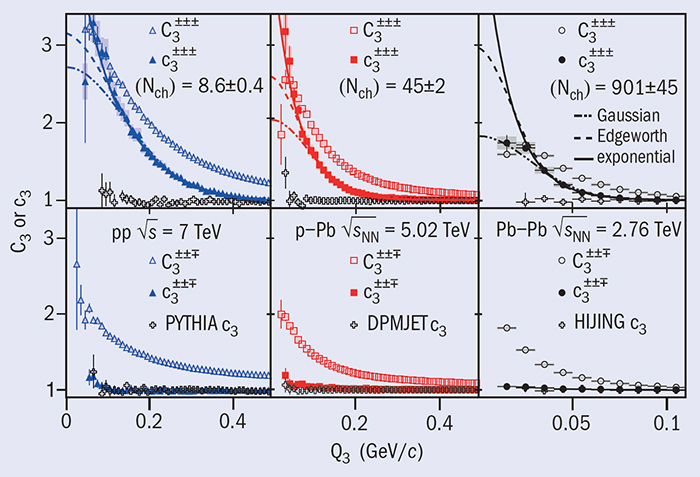
From the measured distributions, the full three-pion correlation function (C₃) can be formed and projected onto the relative momentum variable Q₃ = √(q₁₂² + q₃₁² + q₂₃²), as shown in figure 1, where the invariant relative momentum of a pair is defined as q_ij = √(– (p_i – p_j)^μ (p_i – p_j)_μ). The figure shows the cumulant correlation function (c₃), which subtracts the second distribution as described above, to remove two-pion correlations. The top panels are for same-charge triplets, while the bottom panels are for mixed-charge triplets.

Bose–Einstein correlations occur only for same-charge pions, while Coulomb and strong final-state interactions occur for both same- and mixed-charge combinations. The cumulant correlation functions are corrected for these final-state interactions as well as for the dilution from long-lived emitters (resonance decays and secondary contamination). For same-charge triplets, the three-pion cumulant Bose–Einstein correlation is clearly visible, while for mixed-charge triplets the same cumulant correlation function is consistent with unity, as expected when final-state interactions are removed. In addition, for each of the systems measured, the figure shows model calculations that do not take quantum and final-state interactions into account, demonstrating the power of the three-pion cumulants in removing backgrounds.

The extraction of the source radius at freeze-out is done by means of Gaussian, Edgeworth, as well as exponential fits to the same-charge three-pion cumulant correlations. The Edgeworth fit represents a Hermite polynomial expansion of a Gaussian function, and provides generally a good description of the correlation functions. Figure 2 shows the resulting radii from the Edgeworth fits, as a function of charged-particle multiplicity for each of the three collision systems. For comparison, the radius fit parameters from two-pion correlation functions are shown with hollow points.

The regions of overlapping multiplicity for the lead–lead, proton–lead and proton–proton results provide an interesting comparison of system sizes

The regions of overlapping multiplicity for the lead–lead, proton–lead and proton–proton results provide an interesting comparison of system sizes: the lead–lead radii are 35–55% larger than those in proton–lead at similar multiplicity. This observation points to the importance of the initial state as the number of participating nucleons, and the initial size in a lead–lead collision, is clearly different from that in proton–lead and proton–proton collisions. The proton–proton and proton–lead overlap zone suggests that the proton–lead system is only 5–15% larger than the proton–proton system at similar multiplicity.

These quantitative observations in the zones of overlapping multiplicity are well described with initial conditions alone, without the additional expansion from a phase of hydrodynamics. However, the measurements do not rule out the presence of hydrodynamics simultaneously in all three collision systems.