The ASACUSA collaboration has just published a determination of the antiproton charge and mass to an incredible six parts in a hundred million.* How was this impressive precision achieved and why is it significant?
Knowing the exact charges and masses of the protons, electrons and neutrons that constitute matter is evidently of fundamental importance for the entire edifice of particle physics. Furthermore, once we know these, we know, according to CPT-symmetry, the values for the corresponding components of the antiworld. Given the fact that we already know the particle values very precisely, should we even bother making the measurements for antiparticles?
Such an omission could hardly be more risky. The CPT theorem – which says that all observed phenomena will remain unchanged if we replace particles by antiparticles, invert their motions, and reflect everything in a mirror – is based on falsifiable assumptions. In a universe as old and as big as the one we see, there is time and space enough for even minute deviations from perfect CPT symmetry to become observable, perhaps even to predominate.
Warning messages
Nature even seems to be sending us warning messages in this respect: having provided a full kit of parts for making a large scale universe that is matter-antimatter symmetric, the one that it in fact assembles from these parts is completely asymmetric. Of course we have explanations for this imbalance, but they are not beyond question. Even worse, the CPT theorem itself rests, as T D Lee notes, “on a foundation which has to be unsound, at least at the Planck length (10-33 cm – the measurement precision when quantum fluctuations begin to have gravitational implications), and maybe at a much larger distance” (T D Lee 1995 The Discovery of Nuclear Antimatter Italian Physical Society Conf. Proceedings vol. 53 eds L Maiani and R A Ricci). The symmetry between matter and antimatter, he concludes, “must rest on experimental evidence”.
How then can we measure the antiproton charge, Q, and mass, M, with very high precision? For the proton, as few particle physicists realize, the charge is measured by taking an acoustic cavity containing sulphur hexafluoride and trying to make it “sing” in tune with an oscillating electric field. The extent to which it does not can then be interpreted as a limit on the net charge of bulk matter: if the proton’s and the electron’s charges were not very close, sulphur hexafluoride would sing louder than it does.
In the case of electrons the charge, e, is no longer obtained, as one might think, from a Millikan-type oil drop experiment, but by combining measurements of the Josephson constant, e/h, and the fine structure constant, a, which appears as a scale factor for all energy levels in the hydrogen atom and is proportional to e2/h. That way, not only e but also h, the Planck constant, can be determined.
As antisulphur hexafluoride is not exactly common on Earth (and also for want of a suitable container for it), we must look elsewhere for a value of the antiproton’s charge. The electron e/h and e2//h experiments give us a clue as to how this can be done.
Some years ago the antiproton’s Q/M value was measured relative to that of the proton’s by the Harvard group at CERN’s LEAR low-energy antiproton ring (R A Ricci 1999 Phys. Rev. Lett. 82 3198) to the staggering precision of 9 parts in 1011. This value was not deduced from measurements of the curvature of its trajectory in a magnetic field (such a measurement could never be made with a better error margin than a few parts per thousand) but by tickling it with microwaves to determine its cyclotron frequency, Q/M ¥ B, in the field B.
In physics we build on what we know, not on what we don’t know, so we are not allowed to assume that unknown CPT violations do not scale Q and M proportionately, leaving Q/M unchanged. The question of values for the charge and mass individually was therefore still open. An independent measure of some other combination of Q and M was needed, just as the fine structure constant gives a different combination of e and h above to the one given by the Josephson constant. What better than the Rydberg constant of the antiproton, which is proportional to Q2M?
For this we need an atom in which the antiproton orbits a nucleus, as the electron does in hydrogen. A good candidate (indeed the only one available at present) is the antiprotonic helium atom (an antiproton and an electron orbiting an alpha particle nucleus), easily created by stopping antiprotons from CERN’s antiproton decelerator in helium gas.
By probing this atom with laser beams, ASACUSA can measure a number of optical transition frequencies between pairs of antiproton orbital states with principal and angular momentum quantum numbers (n, L) differing by one (see “Thinking about antiprotonic helium” below). In sharp contrast with the case of electrons in ordinary helium and of hydrogen, these take values around 35-40 when the almost stationary antiproton is captured into an atomic orbit by a helium nucleus (see “Thinking about antiprotonic helium” below). Every such transition of the antiproton in this atom has the antiproton Rydberg constant as a common scale factor.
Now, of course, much of the art of high-precision experimentation lies in accounting for small systematic errors. Stopping the antiprotons in very cold (6 K) helium reduced those due to the Doppler effect severely. The major remaining systematic effect was the so-called density shift arising from the buffeting that the antiprotonic atom suffers from neighbouring ordinary helium atoms. On the theoretical side, the difficulty is that antiprotonic helium is a three-body system, not a two-body system like hydrogen, requiring sophisticated computer calculations.
Among the many transition frequencies measured, the experimenters therefore selected those with the most favourable experimental and theoretical conditions. Instead of trying to work out a value for the Rydberg constant, and combining it with the Q/M value, the equivalent procedure was adopted, asking the theorists to estimate how much the proton values for Q and M used in their calculations had to be changed to give the experimental frequencies, under the 9 parts in 1011 constraint given by the Harvard Q/M ratio. This could be interpreted as a confidence limit on the charge and mass relative to those of the proton.
The result was that if there is any difference between the antiproton Q or M and the proton’s value, it is, with a 90% confidence level, less than 6 parts in 108. This constraint is about 10 times as tight as that obtained by the same procedure at LEAR and a thousand times as tight as that obtained without using antiprotonic helium.
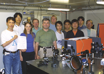
Can we stop here? No. As has been often pointed out, in science we can never verify concepts (like CPT symmetry) with absolute finality – there is always the possibility that still more precise measurements, or measurements of new quantities, will falsify them. This is why the ASACUSA group is now planning further improvements to its laser system that will push the limit to a few parts in one billion, and why it is now also measuring the magnetism of the antiproton to a few parts in 105 or better by flipping the electron’s spin in its orbital magnetic field. The first results are being displayed prominently in the photograph by Hiroyuke Torii of Tokyo.
Thinking about antiprotonic helium
A useful starting point for thinking about antiprotonic helium is the semiclassical picture of the Bohr hydrogen atom usually presented in undergraduate textbooks. It has now been established that if the antiproton approaches an ordinary helium atom slowly enough, it readily replaces one of its electrons, entering an orbit with the same semiclassical radius (some 105 nuclear radii – well beyond the range of annihilation – producing strong interactions) and therefore the same binding energy of about 39.5 eV.
As a first approximation we assume (as is also done in textbooks for ordinary helium) that it does not interact with the remaining electron, but that this nevertheless partially screens the nuclear charge to the value 1.7e instead of 2e. This approximation is adequate to reveal the general properties of the spectrum.
The total (kinetic plus potential) energy in such hydrogen-like atoms is quantized with energy levels En = -ER/n2, where ER is the energy equivalent of the antiproton_helium Rydberg constant. Doing the calculations we then easily find that n is about 38 for En = 39.5 eV, and that the de Broglie wavelength of the antiproton is n times smaller than that of the electron (0.05 nm), justifying our semiclassical assumption. The electron itself is fully quantum mechanical as it was before the antiproton approached.
The figure “Energy levels” shows a schematic energy level diagram for the atom. Evidently the antiproton is in a very highly excited state. Hold the figure vertically in front of you and the n = 1, L = 0 ground state energy of about -60 keV will be found way off the page to the left and a few hundred metres underground!
Now one might have thought that if, during its nanosecond-long approach to the atom, the antiproton had been able to displace the first electron so easily, it would within a few more nanoseconds just as easily have ejected the second one and that the atom (right thumbnail sketch) would quickly become a positive ion (left thumbnail sketch).
The most important characteristic of this atom is that energy and angular momentum conservation prevents this from happening, at least immediately. Instead, the antiproton de-excites spontaneously (black arrows) through a chain of metastable states, emitting optical-frequency (2 eV or 600 nm) photons as it goes with microsecond-scale lifetimes.
Only when it arrives at one of the red states do the energy and angular momentum transfers become favourable for removing the second electron and so for changing the neutral atom into a positive ion. Once this happens the antiproton’s fate is sealed – such ions are very unstable in collisions with ordinary helium atoms, and these soon send the antiproton into the nucleus, where it annihilates.
ASACUSA’s trick is to stimulate transitions to green states with a tunable laser beam, and to detect the resonance condition between the laser beam and the atom by the ensuing annihilation.